COMPARING TWO ALTERNATIVE POLLUTANT DISPERSION MODELS AND ACTUAL DATA WITHIN AN ENVIRONMENTAL HEALTH INFORMATION PROCESSING SYSTEM (EHIPS)

BORIS BALTER, M. STAL'NAYA, VICTOR EGOROV

Space Research Institute, Russian Academy of Sciences
Profsoyuznaya 84/32,
Moscow, 117810,
Russia

Abstract

This paper presents the test results for an air pollutant dispersion modelling unit working within a larger software system EHIPS designed for environmental health information processing. We start with the description of the whole system and then proceed to the modelling unit, which uses two standard dispersion models - one Russian (OND-86) and one American (ISC3ST). The peculiarity of this unit is just in its links to other components of the system, which opens the way to multifold usage of the modelling results, including easy comparison between the model and the data obtained from actual measurements.
We compare the two models and actual measurements on the basis of a one-year data set obtained in an industrial city (Cherepovets, RF). The overall agreement between all three may be characterised as satisfactory. Our interest lies primarily in analysing the dependence of discrepancies between the models and between models and data as a function of pollutant, time, etc. We also discuss the influence of expected deficiencies in pollutant source data on accuracy of modelling. We try to draw lessons for interpreting the risk assessment figures obtained through modelling.
What is EHIPS

In a narrow sense, EHIPS is the software that processes data and model calculations related to the chemical pollution of environment and population health status.
The main features are:

In perspective, EHIPS will also:

The primary users of EHIPS are the official organisations entitled to control of environmental status and related health effects: SanEpid, Ecological committee and municipal administration. The primary uses of EHIPS for them are:

What Problems Addresses EHIPS?

There exists a lot of software for environmental problem analysis: pollutant dispersion modelling, health risk calculation, environmental epidemiological studies etc. However, each software addresses just a specific aspect of data processing. In contrast, EHIPS was designed to connect these multiple aspects and to make one way of data analysis build on another. This drive toward universality can help in the following problems.
Usually, the software made for regulatory purposes (e.g., compliance check) uses some fixed algorithm to calculate concentrations and risks, fill data gaps and so on. However, environmental issues are scientifically intricate and usually need much experimenting and data fitting to obtain a defensible result. Such scientific analysis is supported by completely different software, if at all. EHIPS synthesises regulatory calculation thread and scientific analysis thread. The latter set parameters for the former and, in its turn, checks the results and, if necessary, adapts parameters.
EHIPS does not call for creation of special monitoring systems. It is oriented towards standard databases that exist in Russia on pollutant emissions, measured concentrations, morbidity, mortality etc. Such data mostly lie dead or are used very superficially because before they can be effectively used, they need a lot of preparatory checking, linking to other data, fitting into a specific problem framework. EHIPS brings data deposits back to life by providing a flexible interface (checked on several dozen types of Russian databases) through which data are imported into the universal processing engine and thus are made active.
All types of data mentioned above have a common set of basic operations:

Universal statistical analysis packages support such operations for any type of data, but they contain no specific environmental 'machinery'. In contrast, environmentally oriented packages are normally confined to specific types of data, so that, e.g., mapping operations are not readily extensible from concentration contours to morbidity statistics. EHIPS standardises handling of diverse data types by embedding each in a 'dataspace' with the following 'axes':
Each axis is hierarchically organised. All charting, mapping, statistics, etc. is independent on dataspace choice. Thus, EHIPS is potentially a standardisation tool for environmental analyses.
Normally, environment-oriented software uses either results of direct measurements or results of computer simulation, but not both. However, none of the two is beyond doubt, and it is advisable to use them concomitantly, for mutual check and adjustment. By supporting this regime, EHIPS provides for verifiability of results.

EHIPS Development Status

EHIPS was initiated in 1995 by the environmental modelling group in the Space Research Institute, Russian Acad. Sci., Moscow. In 1996 - 1997 the work was continued by the same group and some additional staff in the framework of RF Environmental Management Project (EMP), and in 1997 - 1999 again by the Space Research Institute.
Three configurations of EHIPS have emerged:
The first configuration is basically ready for installation, the third one exists only in a design document, and for the second one, some work has been done and some not.    Presently, the federal SanEpid officials consider EHIPS as an option for a standard nation-wide tool for environmental health data analysis within local SanEpid services. Before that, EHIPS yet has to pass the necessary testing and certification stages.
Functions

The main functions of EHIPS are as follows.

In contrast to the functions above, the model construction and model parameter setting belongs to the research thread of EHIPS. It includes empirical models, like regression, physically based models, e.g. pollution dispersion, and models that embody the expert judgement, e.g. risk formation and risk expression in morbidity. All these types are treated in a unified manner: model predictions are compared to actual data and the model parameters are obtained from the best fit. This can be done automatically or by experts. The models are used to generate 'simulated' data, which are then processed into hotspots, priorities, etc. Some results of model fit (e.g., pairs of tightly correlated environmental and health indicators) are a direct output for decision-makers, since it helps to identify hazards.
Uncertainty estimation is an ancillary function, which accompanies all stages of data processing. It combines all sources of uncertainty: statistical variation, model inaccuracy, data errors, etc. It finally produces the quality index for EHIPS output information.

Source Data

The following databases should exist for the territory of interest and for at least 1 year.
In the minimal configuration of EHIPS, some of these databases may lack and be substituted by model calculations.
In the maximal configuration, the following additional databases should be present:
The data sources of EHIPS are shown in Figure 1.

Figure 1. Source data and dataflows in EHIPS. Gray squares: federal-level data; white squares within: regional-level data. Rectangles outlined in bold are main processing units each specialised to a data type and forming an information processing pipeline. Within each unit variables are listed across which data are unfolded in the unit. Below: forms of processing output.

EHIPS Structure

EHIPS consists of sequentially linked modules, one for each data type. Presently, there are 5 modules for emissions, concentrations, risks, morbidity and mortality. Extended EHIPS structure will include also modules for integral indices of health loss, related economic loss, cost/benefit criteria, choice of control measures, control implementation plan, and technological processes that lead to pollutant emission.
The background data processing consists in exchange of information between modules. Normally the data is passed along the module sequence, transition between modules being performed by models (e.g., from emissions to concentrations by the pollutant dispersion model; from concentrations to risk by the exposure model, etc.). In a module, the model calculations are harmonised with the measurements taken from databases linked to the module, and then passed on. In extended EHIPS, this process includes the choice of emission control measures, after which the calculation starts with new emissions. Thus, the cycle is closed and runs in circle until a steady state is reached so that a plan of control and respective evolution of hazard are obtained. On this background, EHIPS builds up its functions described above. They are performed by the functional blocks that work with all data modules on equal footing. There is the data overview block that performs tabulating, charting, mapping; the statistical block that performs correlation, regression, cluster and pattern analyses and so on.
Finally, EHIPS includes the service modules that perform links to databases, form the output document, support the network data exchange, etc.
The backbone structure of EHIPS in minimal configuration is shown in Figure 1. The information flow in the maximal configuration of EHIPS is shown in Figure 2.
Dispersion Modelling Unit in EHIPS
Dispersion modelling in the minimal version of EHIPS includes only propagation of flue in air (see upper left part of Figure 1). So, it is just a tiny part of overall data flow. Still, it is important because there is a well-studied physical process behind it. So, it should serve as a template for modelling and model validation.
We use two concurrent models of flue dispersion: ISC3ST developed by US EPA and OND-86 developed by Russian Voeikov Geophysical Observatory. Both are used for regulatory purposes in respective countries. There are many minor differences in scientific approach between these models; the major difference is that ISC uses Gaussian approximation of plume profile from the start, while OND introduces it postfactum, after reducing differential equations of propagation to algebraic form.
The general structure of both algorithms is the same, and it is shown in Figure 3.

Figure 2. Information processing flow in EHIPS.

The major practical issue is that OND is targeted at calculation of absolute concentration maxima at the worst meteorological conditions, while ISC can predict concentrations for any current meteorological situation and is therefore more fit for short-time monitoring and forecast. However, this limitation is not inherent in the OND algorithm, and we extended it using the original description of OND equations so that the two models can be compared at the equal footing. Still, there remains a degree of freedom in transferring the atmospheric stability index between the two models, and this can sometimes change the result by as much as the factor of 2 or 3. Therefore, rather than sticking to absolute values, we paid most attention to the behaviour of model predictions across time, space, and other 'unfolding variables'.


Figure 3. Parameterisation and information flow structures common for ISC and OND. Arrow thickness indicates the relative weight of dependence between parameters it connects.


Results of Modelling

In the following figures we present an example of colour-coded concentrations calculated on a grid of square cells that cover the residential area of Cherepovets City. Colour codes can be read off the scale above the map. The small icons to the upper left of the grid represent the flue emission sources within the largest plant in the city: the Severstal steel plant. However, there exist also other emission sources which can contribute significantly (at least for certain locations and certain pollutants). In addition, flue emission rate was taken from yearly reports rather than from actual measurements on the stack. All this amounts to a considerable uncertainty about emission sources. Therefore, model comparisons to measured concentrations should be 'handled with care'.
Figure 4. ISC3ST: yearly averages of four-times-a-day NO2 concentrations calculated from current meteo. Figure 5. OND-86: yearly averages of four-times-a-day NO2 concentrations calculated from current meteo.

We see that the absolute values consistently differ by approximately a factor of 2, but there is an obvious similarity in the spatial pattern. Its most important feature is a hotspot aside from the flue 'mainstream' - in the northern residential area (more pronounced in OND). Its presence was important for regulatory purposes and also correlated with the higher concentrations measured in this area.

Comparisons

For comparisons between models or models and data we use the tabular/graphics units of EHIPS to which we feed the concentrations. A set of concentrations (say, from one model) is chosen as a reference frame, and another similar set (from another model or from actual data) is plotted with respect to this frame across time, or some other unfolding variable, or turned into a histogram. As a result, we obtain an overview of discrepancies between models or between a model and actual data. Some examples are shown in Figure 6 to Figure 11. (We also introduced some filtering to remove suspected outliers). In these calculations, we used ISC3ST. The range of ratio values is approximately 0.1 - 10. The figures are captured directly from the program's screen so inscriptions are in Russian. See figure captions for explanations.
For most pollutants, model concentrations are considerably lower than measured. That is partly attributable to an incomplete list of pollutant sources. We can make the reasons for discrepancy more clear by unfolding the model/data ratio across time since different sources behave differently in this respect.
For NO2, in summer months, the model is almost exact (ratio close to 1) and in winter it considerably underestimates concentrations. This is probably because thermal power plants used for heating, which were unaccounted for in the model, are not operational in summer, and in winter they are a major source of NO2.
For CO, the models underestimate of concentrations has no obvious seasonal dynamics. This is probably because a large part of CO is due to transport (unaccounted for in the model), which has no pronounced seasonal dependence.
For dust, the model, on the average, was almost exact. That was expected because there were no major sources of dust outside the industry. Interestingly, there were events when measured concentrations were less than modelled. One possible explanation for that lies in the variation of emission intensity (temporary decreases).
As an example of data viewing options, we give the same ratio averaged over a whole city district, now not as a histogram, but as a ranking. In this way, we can quickly identify the largest discrepancy events, to study them in detail.

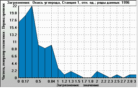
Figure 6. Ratio of modelled CO concentration to actual data (X-axis). Histogram of 4-times-a-day values over 1 year (Y-axis: occurrence per year). Monitoring station 1, year 1996.

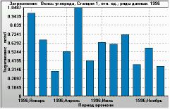
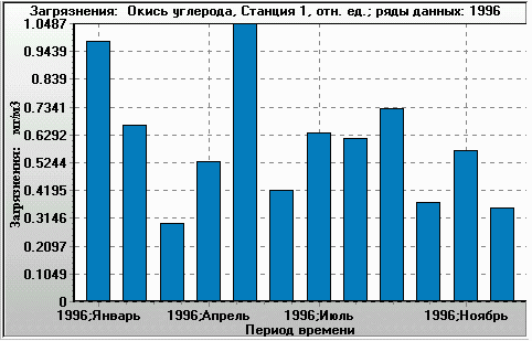
Figure 7. Monthly time series for the same ratio (plotted as Y-axis). X-axis: 1996, January to 1996, December. Monitoring station 1, year 1996. The filtering used was the same as in the histogram.

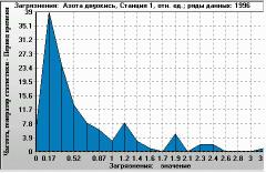
Figure 8. Ratio of modelled NO2 concentration to actual data (X-axis). Histogram of 4-times-a-day values over 1 year (Y-axis: occurrence per year). Monitoring station 1, year 1996.

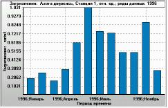
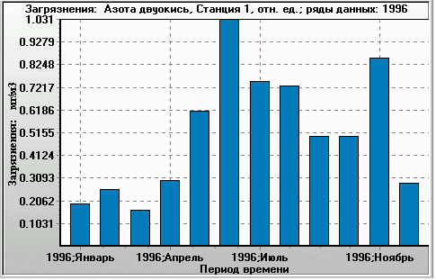
Figure 9. Monthly time series for the same ratio (plotted as Y-axis). X-axis: 1996, January to 1996, December. Monitoring station 1, year 1996.The filtering used was the same as in the histogram.

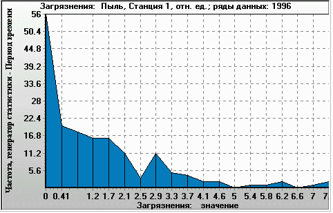
Figure 10. Ratio of modelled dust concentration to actual data for a single monitoring station (X-axis). Histogram of 4-times-a-day values over 1 year (Y-axis: occurrence per year). Monitoring station 1, year 1996.

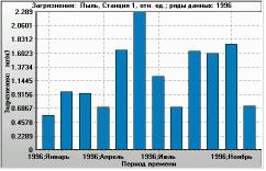
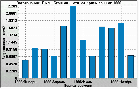
Figure 11. Monthly time series for the same ratio (plotted as Y-axis). X-axis: 1996, January to 1996, December. Monitoring station 1, year 1996. The filtering used was the same as in the histogram.

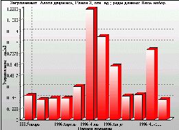
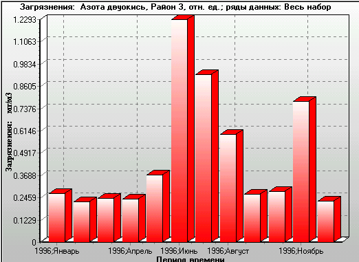
Figure 12. The ratio of NO2 model concentrations to measured data averaged over a city district (plotted as Y-axis). X-axis: 1996, January to 1996, December. City district 3, year 1996. Monthly averages of four-times-a-day ratios.

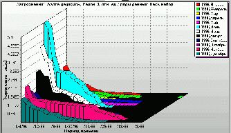
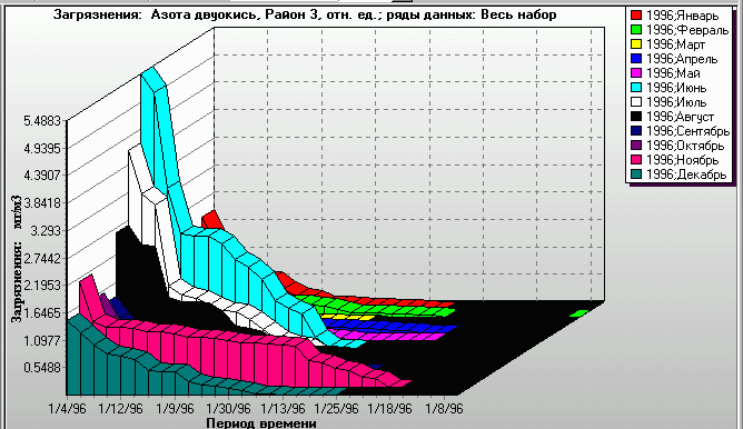
Figure 13. The ratio of NO2 model concentrations to measured data (plotted as Y-axis) averaged over city district 3 (monthly ranking of four-times-a-day ratios). X-axis: days of the respective month ranked highest concentration ratio first.

Another direction of study was the comparison between ISC and OND. As shown in Fig.12, for NO2, the models give comparable results 'on the average' but discrepancies by a factor of 2 are not unusual. That is primarily due to sensitivity of results to modelling details when the cell, for which modelling is performed, is on the plume's tail. Once more, as seen in Figure 5, the spatial patterns are very much the same for both models.

Using the Results

The primary use of model concentrations in EHIPS is for health risk assessment. We are primarily interested in non-cancer risks for which standard risk assessment schemes do not provide a good estimate. EHIPS uses for that a special risk model developed by Prof. S.Novikov. It combines inputs from all calculated non-carcinogeneous pollutants. The resulting risk map is shown in Figure 14. It is calibrated so that zero risk corresponds, roughly speaking, to non-observable effect level, and the risk equal to 1, to death outcome. As shown in the histogram of daily risks (Figure 15), the prevalent input is formed by the dust, which is known to be related to total mortality.
Note that, due to overlapping of spatial patterns for several pollutants, the risk pattern is slightly different from those shown in Figure 5 etc. The northern hotspot took the form of an elongated 'concentration ridge'.
Figure 14. Noncarcinogeneous risk displayed on the city plan: 1-year average of daily values calculated from ISC3ST model. Top: color scale for relative risk index. Colored squares: cells of calculation grid. Square icons: emission sources, icon showing the type. Black squares: industrial buildings. Figure 15. Noncarcinogeneous risk: 1-year histograms of daily risk values (plotted as X-axis) calculated from the ISC3ST model for major measured pollutants. The list of pollutant color codes (top right): NO2; no data; NH3; no data; no data; CO; dust; H2S; no data; phenols; formaldehyde; SO2. Yearly occurrence of daily risk values plotted as Y-axis.

Discussion

We have drawn the following preliminary conclusions from our modelling experiments in EHIPS.
  1. OND and ISC give compatible yearly averages but can diverge by the factor of 2 to 3 in one-shot estimates. They can be used concurrently for mutual check.
  2. Even if models underestimate actual concentrations considerably, they can give reproducible (and hence, hopefully, correct) spatial and temporal patterns. Therefore, they can be corrected to actual measurements so as to 'interpolate' between sparse measurement points.
  3. There can be stable hotspots in unexpected locations, and model-based risks in adjacent modelling cells may differ by a factor of 2.

Contacts

For additional information and documentation please contact EHIPS team through:
Balter Boris Mikhailovich: ehips@yandex.ru (495)333-4467
Egorov Victor Valentinovich: ehips@yandex.ru (495)333-3589

References

View the EHIPS Website (mostly in Russian) at http://www.iki.rssi.ru/ehips/welcome.htm