| |
Abstract
This is a systematic attempt to identify and assess near-equatorial, high-eccentricity orbits best suited for studying the Earth's magnetosphere, in particular its most dynamic part, the plasma sheet of the magnetotail. The study was motivated by the design needs of a multi-spacecraft "constellation" mission, stressing low cost, minimal active control and economic launch strategies, and both quantitative and qualitative aspects were investigated. On one hand, by collecting hourly samples throughout the year, accurate estimates were obtained of the coverage of different regions, and of the frequency and duration of long eclipses. On the other hand, an intuitive understanding was developed of the factors which determine the merits of the mission, including long-range factors due to perturbations by the Moon, Sun and the Earth's equatorial bulge.
|
An overview of the Earth's Magnetosphere
The Earth's magnetosphere, the space region dominated by the Earth's magnetic field, provides a unique laboratory for studying large-scale plasma phenomena of astrophysics and geophysics.
It is usually defined as a comet-shaped cavity carved in the solar wind by the Earth's magnetic field, which blocks the solar wind flow. The boundary of that cavity ("magnetopause") is rounded on the day side, where its closest distance to the Earth's center averages 10-11 RE (Earth radii; 1 RE = 6378 km). It is about 15 RE wide abreast of Earth (all distances from the center of Earth) and on the distant night side it tends to a cylinder of a radius of about 25 RE (Figure 1).
Ahead of the magnetopause, in the Sun's direction, a collision-free bow shock forms, typically approaching Earth within 13-14 RE. That shock and the "magnetosheath," the region of shocked solar wind between it and the magnetopause, are also of interest to space plasma research.
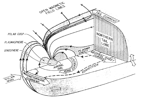
Figure 1. Schematic view of the Earth's Magnetosphere
Many physical phenomena in and around the magnetosphere depend on the configuration of its magnetic field lines (or "lines of force"), since ions and electrons tend to spiral around such lines and thus become attached to them. Field lines on the sunward ("day") side of the Earth are compressed, while those on the night side (the "tail" or "magnetotail" region) are stretched out. The lines of the tail form two long bundles or "tail lobes". Each magnetic field line of course has a definite direction: those of the northern tail lobe are directed into the region around the northern magnetic pole ("northern polar cap"), while those of the southern lobe are directed out of the southern polar cap, away from Earth.
Possibly the most significant region is the "plasma sheet" sandwiched between the two lobes, about 5 RE thick. Compared to the lobes, its magnetic field is much weaker and its plasma much denser. It is the site of many active phenomena, including impulsive "substorms" which energize ions and electrons and drive them earthward. Much of the polar aurora and of the electric currents with which they are associated comes from the plasma sheet.
The dipole-like inner magnetic field, near Earth, traps the Earth's radiation belts. The ions and electrons of the outer belt are merely the high-energy end of a much more extensive particle population named the "ring current," from the electric current which it carries, which modifies the field arising from the Earth's interior. Ring current particles typically fill the region from 3 to 9 RE and originate in magnetic storms and substorms. The inner radiation belt, in contrast, is confined to a compact region near the magnetic equator (at distances of 1.3-2.5 RE) and contains high-energy protons, a by-product of the cosmic radiation. Its magnetic effects are much weaker than those of the ring current, but it is dense enough to cause gradual radiation damage to any satellite that spends appreciable time in it, in particular to the solar cells that power such satellites.
For additional details, see Stern and Ness [1982] and also, on the world-wide web, Stern [1995],
Missions to Study the Magnetosphere
Many unmanned spacecraft have in the past studied the Earth's magnetosphere, notably the IMP series, the ISEE, DE and AMPTE missions, and more recently Geotail, Polar, Wind, Interball, Explorer-S and Image. While most past missions have used single spacecraft or paired ones, future missions are likely to use networks of multiple satellites, starting with "Cluster" in mid-2000.
This investigation, too, arose from the study of a "constellation" of multiple spacecraft. Named "Profile" (Stern, [1998a, b]) that mission proposes to observe (among other things) near-radial profiles of the magnetosphere, using 12 small satellites spaced one hour apart on two slightly different orbits. This article describes what that study found about the selection of single satellite orbits for studying the distant magnetosphere; a later article will focus on the multi-satellite aspects of such missions.
Space missions are inherently expensive and difficult. It is therefore quite important to identify orbits which give the best scientific returns. For magnetospheric missions, eccentric orbits with high apogee are often the best (see criteria listed further below), because the active regions of the magnetosphere--in particular, the plasma sheet and magnetopause--lie beyond 10 RE, while a low perigee makes data down-loading easier. The orbits of ISEE 1/2, a close pair with apogees around 23 RE, may be viewed as typical of this class. Here we consider only low inclination orbits, best for the plasma sheet. Missions with steeply inclined orbits like those of Polar and Interball form a different class, useful for examining the region around the polar cusps, where field lines closing on the day side are separated from the ones swept into the tail.
The missions considered here tend to have multiple goals, because during the year, as Earth orbits the Sun, the axis of the spacecraft orbit, nearly fixed in inertial space, rotates around the magnetosphere, whose axis follows the direction of the Sun and of the solar wind. If at some time the orbital axis passes the plasma sheet, 3 months later it is directed to the flanks and 3 months after that it will be in the noon sector.
Coordinates
Three Cartesian coordinate systems are used in this article, all of them geocentric. Each is defined by two of its coordinates, with the third defined by completing a right-handed triad.
- Celestial coordinates (x, y, z), with z pointing northward along the Earth's spin axis and the x axis aligned with the line of intersection between the equatorial plane of Earth and the plane of the ecliptic, in the direction of the vernal equinox.
- Geocentric ecliptic coordinates (xe, ye, ze), with xe = x but ye in the plane of the ecliptic.
- Geocentric solar-magnetospheric (GSM) coordinates (xSM, ySM, zSM), with xSM pointing into the flow of the solar wind (a direction approximated by the one to the Sun) and the (xSM, zSM) plane containing the Earth's magnetic (dipole) axis.
Tail Hinging and Warping
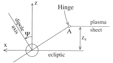
The most critical coverage in missions of the above class is that of the plasma sheet. Different choices of orbital elements affect only slightly the coverage of the flanks and of the dayside (see Table 4, later on) but not of the plasma sheet. The main complicating factor is the deformation of the plasma sheet due to the varying tilt angle Ψ, where (90°–Ψ) is the angle between the Earth's dipole axis and a vector pointing into the flow of the solar wind, approximated by the sunward direction (Figure 2a).
When the Earth's magnetic axis is perpendicular to the sunward direction (as happens near equinox), the magnetosphere has north-south symmetry. The plane of symmetry is also the "magnetic equatorial surface," the collection of points where on any field line is the furthest from Earth. For non-zero Ψ, however, that surface is deformed: near Earth it follows the (inclined) magnetic equatorial plane, but past 7 RE it gradually bends over and aligns itself with the flow of the solar wind (Figures 2a).
|
Figure 2a. The hinging of the midnight plasma sheet, due to the tilt angle Ψ of the Earth's dipole axis, schematically shown in the (xSM, zSM) plane of GSM coordinates.
|
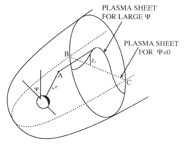
Near midnight, the effect can be approximated by following the direction of the magnetic equator up to a "hinging point" A at about 8RE, then continuing in the anti-solar direction (Figure 2a). Away from the midnight meridian the surface is further deformed by the requirement (a consequence of pressure balance) that the two tail lobes should have approximately the same cross-sectional areas. As a result, away from midnight the hinging point moves closer to the (xSM, ySM) plane and as Figure 2b shows, and near the flanks it actually crosses that plane to its side opposite from A.
The shape of the warped plasma sheet was derived here using formulas obtained by Tsyganenko [1995]. The likelihood of an observation point being in the plasma sheet (an important scientific criterion--see below) depends mainly on the distance Δz from the deformed equatorial surface. The shape of that surface, in GSM coordinates, can be defined by an equation zs = zs (xSM, ySM,Ψ); various approximations exist for the observed variation of zs and one of them was used here, in a FORTRAN subroutine NSHEET.
|
Figure 2b. The warping of the plasma sheet away from the midnight meridian, schematically shown in GSM coordinates.
|
Metrics and Methods
Effective planning of a magnetospheric mission requires the following "metrics" (quantitative measures):
- Criteria for evaluating a desirable orbit. These may include trade-offs that allow one to strike a compromise between desirable and undesirable features.
- A list of variables whose choice determines the orbit.
- A method of evaluating an orbit, to decide how well it answers the mission's needs.
Using those quantitative metrics, one next seeks to find optimal orbits. Two approaches exist here:
- Try out a large number of orbits, examine them, deduce trends which improve performance, then follow those trends until no further improvement is obtained, or until the trade-off with undesirable features is as good as can be expected. That has been the usual approach in the past.
- Try to explicitly identify the factors which determine the merit of the mission, as defined above, and use them to identify the region in parameter space where "good" orbits are expected to exist. That approach was used here.
Metrics for Planning the Mission
(A) Criteria for a Desirable Orbit
- Economic spacecraft. The "Profile" mission envisioned small inexpensive satellites, spin stabilized (see #6 below) and requiring no on-board propulsion.
- Economic launch. The thrust required to achieve an orbit with a given apogee is reduced when perigee is as low as possible. At the same time, a highly elliptic orbit (apogee 20-25 RE or more) suffers significant perturbations due to the Moon and Sun. Such perturbations keep the semi-major axis invariant, but other orbital elements vary. Decreases in eccentricity, in particular, lower perigee height and can cause premature reentry.
- Good coverage of the plasma sheet in the geotail, which requires low inclination to the ecliptic. The mission may also envision observations in the near-equatorial dayside and flanks, but these (as shown in Table 4) are largely orbit-independent.
- Avoidance of extended eclipses, which can damage the spacecraft by excessive chilling. Eclipses near Earth, up to one hour, can hardly be avoided: the danger is posed by eclipses near apogee, where the satellite moves slowly and may spend up to 9-10 hours in the Earth's shadow.
A small orbital inclination to the ecliptic, which favors plasma sheet coverage (#1 above) also makes distant eclipses more likely (at the time of the year when perigee is near noon). Obviously, some compromise is needed.
- Long orbital lifetime. The lifetime of ISEE 1/2 was about 8.5 years, which is about as long as an extended mission might last. Perhaps equally important, as time goes on and perturbations modify the orbit, adherence to criteria #3 and #4 above should not deteriorate.
- The most desirable spin axis is one perpendicular to the ecliptic, which allows the plasma instrument to compare ion fluxes in opposite directions in the plane of the ecliptic. That plane is close to the equatorial surface of the plasma sheet, and from this plasma bulk motions along that surface can be deduced.
Such a spin also helps sample the solar wind when outside the magnetopause, and in a cylindrical satellite it assures an even illumination of solar cells. We give up on any propulsion, because it would have to be along the spin axis, approximately perpendicular to the orbit plane.
- Avoidance of the inner radiation belt, which can damage the spacecraft and in particular degrade its solar cells.
That desirable feature, unfortunately, contradicts others, described earlier, and was in the end considered expendable. To avoid the inner belt, perigee would have to be raised to 3 RE or higher, but the greater range would require either increased transmitter power, a reduced data rate and/or large tracking antennas. It would also make it hard to deorbit the s/c after the mision is complete, to avoid creating space debris. Alternatively, solar cells could be protected by a 1 mm glass cover, and an extra margin of 25% in the available power could be added to compensate for their gradual degradation. The electronics and instruments can also be designed to survive the radiation, which (for the solar cells, the most exposed part) may amount to 25 rad per pass.
(B) Parameters that Determine the Orbital Elements
Given an available launch capability, the resulting orbit is determined by the following adjustable parameters:
(a) Time of the day of the launch.
(b) Day of the year of the launch.
(c) Year of the launch
(d) Option of entering a parking orbit and delaying the
firing of the last rocket stage.
(e) Location of the launch site
(f) Direction of the launch azimuth, other than eastward.
In early studies, only options (a)-(d) were considered, but with options (e) and (f) added, greatly improved orbits are feasible.
(C) Evaluation of Magnetospheric Coverage
The evaluation of orbits requires:
(a) A realistic model of the magnetosphere.
(b) Simulations of actual orbits, using the above criteria and the magnetosphere model to estimate the time spent in each region. Such simulations can also estimate the number and duration of distant eclipses, and answer other questions.
Average boundaries of magnetospheric regions were calculated as follows. For the magnetopause we used equation (2) of Sibeck and Roelof [1991], and for the location of the bow shock the equations of Fairfield [1971]. The equatorial surfaces in the tail, depending on the tilt angle Ψ, were approximated as described earlier. On the night side, the inner boundary of the plasma sheet was approximated by the dipole field line crossing the magnetic equator (equidistant from the magnetic poles) at a distance r=8 RE. The region between that and the dipole line with rPS=6 RE, was deemed as "transition region" to the inner magnetosphere.
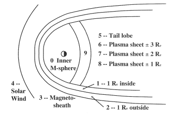
Each position (x,y,z) of the satellite's orbital simulation was converted into GSM coordinates. After that, a subroutine MSREG used the above criteria to assign the point to one of 10 regions (Figure 2-c), using index IREG = 0 to 9, as follows
|
Figure 2c. The classification of magnetospheric regions used in this study.
|
| IREG |
Region |
IREG |
Region |
|
0 |
Inner magnetosphere |
5 |
Tail lobe
|
|
1 |
0-1 RE inside magnetopause |
6 |
Plasma sheet, 2 < |Δz| < 3 |
|
2 |
0-1 RE outside magnetopause |
7 |
Plasma sheet, 1 < |Δz|< 2 |
|
3 |
Magnetosheath |
8 |
Plasma sheet, |Δz| < 1 |
|
4 |
Solar Wind |
9 |
Transition region, 6 to 8 RE |
The region around the polar cusp and above the poles was classified by IREG=10, but results are not listed here, because the orbits studied were close to the equator and never reached it.
Simulation of the Orbit
The codes used in simulating the magnetospheric coverage were developed for the "Profile" mission (Stern, [1998a, b]) and therefore simulated not single orbits but groups of 12, differing in mean anomaly and having two slightly different values of the semi-major axis. As a result, the coverage statistics obtained here apply not to isolated missions but to ensembles of 12, which makes the results less sensitive to random fluctuations.
The Fortran code ORB6D3 which conducted the simulations assumed Keplerian ellipses, neglecting slow perturbations by the Moon, Sun and the equatorial bulge of Earth. More sophisticated simulation codes (much slower), based on perturbed orbits, were also developed. However, the output of such codes combines two separate effects on magnetospheric coverage: the choice of orbital elements, and the slow variation of those elements with time; Keplerian simulations isolate the first effect alone. Keplerian codes, using as inputs the osculating orbital elements given by the perturbation code, can estimate coverage later in the mission, with the more sophisticated codes used in the final analysis.
All simulations covered one "short year" of 364 days (=52 weeks). Each hour of the year the position of each satellite was checked and assigned to one of the regions, and weekly coverage statistics were checked, as well as totals for the year and for each 13-week season. In addition to coverage statistics, the code also compiled eclipse statistics for locations with xSM = –2RE, noting which of the satellites was shaded each hour by the Earth and classifying eclipses by the number of accumulated eclipse hours. The calculation assumed the shadow of the Earth to be a cylinder, thus slightly overestimating the severity of eclipses.
Launch from Cape Canaveral
Most space launches by the US are conducted from Cape Canaveral, Florida, at north latitude 28.50, due eastward. That adds to the launch velocity a contribution from the Earth's rotation of about 407 m/sec and assures that the orbital inclination i to the Earth's equator will be 28.50. As an initial simplification, assume that the spacecraft is injected into its orbit right above Cape Canaveral and that its initial perigee is there.
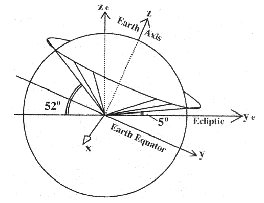
Figure 3. The variation of the orbital inclination ie of orbits launched from Cape Canaveral (lat. 28.5°N), ranging from 5° to 52° depending on the time of day on which the launch takes place. The time when ie is minimal is here the "reference time," and launching at that time puts apogee in the midnight meridian at summer solstice.
|
The radial line to the perigee point will lie on a cone around the Earth's axis, with opening angle 61.50 equal to the co-latitude of Cape Canaveral (Figure 3), Because of the inclination angle ε = 23.5° between the Earth's axis and the ze direction perpendicular to the ecliptic, the orbital inclination ie to the ecliptic on any launch date can be anywhere from (28.5–23.5) = 5° to (28.5+23.5) = 52°, depending on the time of the day when the launch occurs. On any day, we define as the reference time the time when a launch gives ie its minimum value; for an orbit starting at such a time, the right ascension of the ascending node is Ω = 0. The value of ω implied by an orbit starting above Cape Canaveral is 90°; the actual value will differ, depending on the distance down the range where the orbit is achieved. Any other value of &969; may be attained by placing the satellite in a circular parking orbit and firing the last stage after some delay.
Unfortunately, a choice of ω = 90° produces a very poor phasing between the orbit and the hinging of the midnight plasma sheet. Since perigee is then 5° north of the ecliptic, apogee will be south of it. However, as Figure 4a shows, the choice of minimal ie places apogee in the tail at the summer solstice when the axial tilt ε of the Earth's axis gives the midnight sector of the equatorial surface its greatest northward displacement.
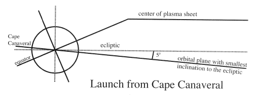
Figure 4a. Schematic view of an orbit launched from Cape Canaveral at the "reference time" (see Fig. 3). Apogee evidently misses the warped plasma sheet, passing on the opposite side of the equator.
|
The average tilt angle Ψ at solstice also equals ε, modulated in a diurnal cycle by about 50% because of the 100 angle between the Earth's magnetic axis and its rotation axis. Because of the hinging effect, the midnight plasma sheet will also be near its greatest northward displacement, while the satellite at its apogee (where much of the mission's time is spent) is south of the ecliptic and is likely to miss it altogether, except near the flanks (Fig. 2b).
Parking Orbits
One way of avoiding this problem is to change ω by first launching the spacecraft into a circular parking orbit, and then after a suitable interval fire the last rocket stage into a final elliptical orbit. The circular orbit determines the orbital plane. Allowing the spacecraft to traverse an angle δ in its parking orbit yields ω = ω0 + δ, where ω0 is the initial value of ω (not necessarily 90° because actual orbit insertion will be east of Cape Canaveral). With ω = 180° the line of apsides is rotated from the (ye, ze) plane in Figure 3 to a direction perpendicular to that plane, parallel to the celestial x-axis. We will call this the "reference orbit."
The reference orbit provides excellent coverage of the plasma sheet. However, by placing apogee in the plane of the ecliptic, it practically assures long eclipses around the time of equinox. To prevent this from happening, the orbit must be "detuned" from that orbit in one of two ways: either by making δ larger or smaller than 90°, or by advancing or delaying the launch by a few hours, relative to the reference time.
Detuned Orbits
Any such "detuning" implies a compromise: eclipses should be tolerably short, while the coverage of the plasma sheet should not suffer too badly. Tables 1a and 1b give the results for a 67 hour orbit (more precisely, for an ensemble of six 66-hour orbits and six 68-hour ones), corresponding to an apogee near 25 RE (perigee is 1.1 RE). Table 1a counts the time in hours spent during the year by the 12 satellites in the plasma sheet, within 1 RE of the equatorial surface, i.e. with IREG = 8. Times with IREG=6 and IREG=7 are comparable. In a short year of 52 weeks, a dozen satellites total 104,832 hours of observation, so as a rough rule, each 1000 hours recorded on that table are equal to about 1% of the observing time. Note that the best coverage is obtained not with the reference orbit but with orbits delayed by 2-3 hours from the "reference time", and with δ = 120°.
Table 1a
Table 1a
Delay →
Coast angle | –2
| –1
| 0
| 1
| 2
| 3 hours
|
|
↓
|
|
50° | 7623 | 5187 | 4263 | 3388 | 3087 | 2380
|
|
60° | 9275 | 7301 | 5551 | 4473 | 3549 | 2954
|
|
70° | 8526 | 7504 | 6272 | 5719 | 4319 | 3514
|
|
80° | 7287 | 7357 | 6524 | 6643 | 5425 | 4165
|
|
90° | 6447 | 7056 | 6370 | 6993 | 6300 | 5054
|
|
100° | 5418 | 6503 | 6223 | 7257 | 7084 | 5915
|
|
110° | 4242 | 5663 | 6181 | 7399 | 8239 | 7210
|
|
120° | 3535 | 4347 | 5474 | 6930 | 8925 | 8876
|
|
130° | 3052 | 3304 | 4172 | 4970 | 7287 | 8603
|
|
140° | 2408 | | 3143 | | 5019 | 6706
|
Table 1a The number of hours spent within 1 RE of the middle of the (warped) plasma sheet by satellites in 12 sample orbits of period 67-hours, launched from Cape Canaveral (apogee near 25 RE; see text for details). Launches are delayed from -2 to +3 hours from the "reference time," and the angles traversed in the parking orbit before the last stage is fired are given in degrees, from 50° to 140°. A score of 1000 approximately equals 1% of the observing time.
|
Table 1b
Table 1b
Delay →
Coast angle | –2
| –1
| 0
| 1
| 2
| 3 hours
|
|
↓
|
|
50° | 6 (31) | 8 (41) | 5 (12) | 2 (83) | 2 (14) | 1 (248)
|
|
60° | 5 (12) | 7 (21) | 6 (10) | 2 (98) | 2 (12) | 1 (248)
|
|
70° | 4(6) 3(54) | 6(4) 5(40) | 7 (22) | 2 (122) | 2 (24) | 1 (246)
|
|
80° | 3 (23) | 4 (41) | 8 (24) | 3 (15) | 2 (52) | 2 (36)
|
|
90° | 2 (82) | 3 (66) | 9 (12) | 3 (59) | 2 (96) | 2 (66)
|
|
100° | 2 (54) | 3 (30) | 8 (31) | 4 (35) | 3 (23) | 3 (12)
|
|
110° | 2 (30) | 2 (117) | 7 (28) | 6(3) 5(35) | 4 (16) | 3 (42)
|
|
120° | 2 (12) | 2 (111) | 6 (14) | 7 (23) | 5(8) 4(45) | 4 (31)
|
|
130° | 2 (17) | 2 (74) | 5 (19) | 9(1) 8(29) | 7(3) 6(40) | 6 (18)
|
|
140° | 2 (30) | | 4 (32) | | 8 (30) | 8 (12)
|
Table 1b Similar to Table 1-a but giving, for the same 12 orbits, the duration in hours of the longest eclipse, and in parentheses, the total number of such eclipses for all those orbits.
|
Table 1b tallies distant eclipses in the same orbits; each cell gives the length in hours of the longest eclipse, and in parentheses, the number of such eclipses recorded for 12 orbits during the year of the run. A few of the entries also record eclipses one hour shorter than the maximum, in general much more numerous, and those shorter by two hours are more numerous still. All these tallies must be divided by 12 to give the average per satellite.
Comparing the two tables shows that orbits with the best plasma sheet coverage also have the longer eclipses. There exist no bargains, only some reasonable compromises. A delay of 2 hours and δ = 60° places the satellites in the central plasma sheet about 3.5% of the mission (or about 10% within 3 RE of the equatorial surface) at the price of one 2-hour eclipse per year. If the mission can annually afford two 3-hour eclipses (and a fair number of 2-hour ones), δ = 100° gives about twice the above plasma sheet exposure.
Table 2a
Table 2b
Table 2a
Delay → | –2 | –1 | 0 | 1 | 2 | 3 hours
|
|
ie | 13.90° | 8.25° | 5.05° | 8.25° | 13.9° | 19.86°
|
|
ωe | –124.1 | –134.1 | –180. | 134.1 | 124.132 | 124.091
|
|
Ωe | –82.98 | –59.37 | 0. | 59.37 | 82.98 | 96.79
|
|
|
Coast angle
↓
|
|
50° | 7672 | 6069 | 4900 | 4550 | 4060 | 3185
|
|
60° | 10255 | 7777 | 6216 | 5229 | 4606 | 3878
|
|
70° | 10514 | 9163 | 7532 | 6797 | 5376 | 4557
|
|
80° | 9296 | 9114 | 8190 | 7994 | 6902 | 5670
|
|
90° | 8414 | 9058 | 8477 | 9233 | 8554 | 7574
|
|
100° | 7399 | 8505 | 8589 | 9912 | 10395 | 9541
|
|
110° | 6006 | 7196 | 8099 | 9632 | 10892 | 11053
|
|
120° | 4585 | 5600 | 6202 | 8050 | 9590 | 10682
|
|
130° | 3297 | 4081 | 4424 | 5243 | 4613 | 8750
|
|
140° | 2835 | 2835 | 3346 | 3654 | | 5824
|
Table 2a Similar to Table (1-a), but for a 47-hour orbit, apogee near 20 RE.
Table 2a
Delay → | –2 | –1 | 0 | 1 | 2 | 3 hours
|
|
ie | 13.90° | 8.25° | 5.05° | 8.25° | 13.9° | 19.86°
|
|
ωe | –124.1 | –134.1 | –180. | 134.1 | 124.132 | 124.091
|
|
Ωe | –82.98 | –59.37 | 0. | 59.37 | 82.98 | 96.79
|
|
|
Coast angle
↓
|
|
50° | 7672 | 6069 | 4900 | 4550 | 4060 | 3185
|
|
60° | 10255 | 7777 | 6216 | 5229 | 4606 | 3878
|
|
70° | 10514 | 9163 | 7532 | 6797 | 5376 | 4557
|
|
80° | 9296 | 9114 | 8190 | 7994 | 6902 | 5670
|
|
90° | 8414 | 9058 | 8477 | 9233 | 8554 | 7574
|
|
100° | 7399 | 8505 | 8589 | 9912 | 10395 | 9541
|
|
110° | 6006 | 7196 | 8099 | 9632 | 10892 | 11053
|
|
120° | 4585 | 5600 | 6202 | 8050 | 9590 | 10682
|
|
130° | 3297 | 4081 | 4424 | 5243 | 4613 | 8750
|
|
140° | 2835 | 2835 | 3346 | 3654 | | 5824
|
Table 2b Similar to Table (1-b) but for a 47-hour orbit. Eclipses are shorter due to the lower apogee.
Of course, any fit tuned so finely is not likely to persist to the next year's apogee pass through the tail, because of orbital perturbations due to the Moon, Sun and the equatorial bulge of the Earth. Tables 2 give corresponding numbers for orbits of 47±1 hours, with apogee around 20 RE. Plasma sheet coverage is typically 30% higher, but these orbits miss the interesting region around 25 RE where (according to many claims) magnetic reconnection in substorms begins.
Launches from points near the Equator
Even the best orbits here are a compromise, balancing plasma sheet coverage against distant eclipses. Fortunately, an alternative exists, providing good plasma sheet coverage without the penalty of long eclipses--namely, by launching from a site near the equator.
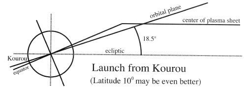
Figure 4b. Schematic view for a launch from Kourou (lat. 5° N) at the "reference time" of its longitude. Now ie is (technically) negative and fairly large, minimizing distant eclipses, but since apogee in mid-summer is placed well north of the ecliptic, plasma coverage is quite good.
|
Such launches may be carried out either from the launch site of the European Space Agency (ESA) in Kourou, French Guiana (lat. 5°N, long. 52.5° W), or from the recently introduced "Sealaunch" ship [Smith 1999a, b] , as well as with the "Pegasus" rocket launched from an L-1011 airplane. The arguments developed earlier for Canaveral launches show that such sites can readily provide orbits with zero inclination ie to the ecliptic. If apogee is then at midnight during equinox (which would require a parking orbit), satellites would be in the plasma sheet essentially all the time they spent on the night side. That would give the greatest possible coverage, but distant eclipses would be frequent, and they would have the longest possible duration, up to 9-10 hours with 25 RE apogee.
What is proposed here is quite different, and assumes launches timed near the "reference time" defined earlier. For orbits launched from Kourou, this would produce an inclination to the ecliptic of ie = 5–23.5 = –18.5°, i.e. perigee will be south of the ecliptic (this corresponds to ie = 18.5°, with ω and Ω shifted by 180°). Because ie is now large, few eclipses are expected in the distant part of the orbit, near apogee.
As shown earlier, orbits launched at the "reference time" (with no delay in a parking orbit) place apogee in the tail during summer solstice, when the midnight plasma sheet is shifted as far north as it can go. Unlike the orbit launched from Cape Canaveral, however, this one has perigee south of the ecliptic, and its apogee is therefore also north of the ecliptic, overlapping the plasma sheet (Figure 4b). In other words, this orbit takes advantage of the plasma sheet's warping to obtain both good coverage and reduced eclipses.
Table 3 compares a number of near-equatorial launches, each calculation combining 12 orbits with periods 67±1 hours, i.e. with apogee near 25 RE. All launches are either at the reference time or with delays of up to several hours, as noted. The assumed longitude is always that of Kourou (–52.5°), but the latitude is either that of Kourou (5°) or as indicated on the table. Two orbits from Cape Canaveral are included for comparison, one of them (#3, marked *) using a parking orbit and delayed firing.
Table 3
Run
|
Lat
(deg)
|
Delay
hours
|
IREG=6
|
IREG=7
|
IREG=8
|
Longest
eclipes
|
Number
|
| |
|
|
1 | 5 | 0 | 6783 | 5873 | 6027 | 1 hour | 252
|
|
2 | 5 | 0 | 6650 | 5880 | 6020 | 1 | 114 |
|
|
3 | 28.5 | 2* | 5670 | 3808 | 3549 | 2 | 9 (286)
|
|
4 | 28.5 | 0 | 4578 | 756 | 56 | 2 | 217 (284)
|
|
5 | 5 | 1 | 7182 | 6076 | 6195 | 2 | 24 (243)
|
|
6 | 5 | 2 | 7679 | 6706 | 6944 | 2 | 78 (126)
|
|
7 | 5 | 3 | 7441 | 7427 | 8197 | 3 | 57 (65)
|
|
8 | 5 | 4 | 6916 | 7854 | 8827 | 5 | 26 (24)
|
|
9 | 5 | –1 | 7308 | 6027 | 6342 | 2 | 24 (243)
|
|
|
|
1 | 5 | 0 | 6783 | 5873 | 6027 | 1 | 252
|
|
10 | 10 | 0 | 7609 | 8995 | 9527 | 2 | 24 (300)
|
|
11 | 15 | 0 | 7448 | 10227 | 11662 | 2 | 76 (331)
|
|
12 | 20 | 0 | 7210 | 6307 | 8470 | 3 | 113 (216)
|
|
|
|
11 | 15 | 0 | 7448 | 10227 | 11662 | 2 | 76 (331)
|
|
13 | 15 | 1 | 7049 | 9821 | 11522 | 3 | 18 (108)
|
|
14 | 15 | –1 | 7035 | 9891 | 11389 | 3 | 12 (108)
|
|
|
|
10 | 10 | 0 | 7609 | 8995 | 9527 | 2 | 24 (300)
|
|
15 | 10 | 1 | 7784 | 8701 | 9954 | 2 | 60 (258)
|
Table 3 Comparison of plasma sheet coverage and eclipse statistics for 15 selected orbits--2 from Cape Canaveral, 7 from Kourou and 6 from intermediate latitudes.
|
For each mission, the table lists the annual number of hours spent in regions 6, 7 and 8 of the plasma sheet, the length in hours of the longest eclipse and the annual number of such eclipses for 12 orbits--counting only eclipes more distant than 2 RE. In parentheses, the number of eclipses one hour shorter than the maximum is also given. For instance, the average satellite in run 5 will experience each year two 2-hour eclipses and about 20 1-hour eclipses. The following features are illustrated by the table:
- Runs #1 and #2 compare two missions from Kourou with the same orbit, except that in #2 the starting positions of all satellites are shifted ahead by 20 hours. That simulates an orbit equivalent but not identical, and the difference helps one estimate random variations expected between equivalent orbits. A variation is evident, but it is small. Note that the longest recorded duration of a distant eclipse is just one hour.
- Runs #3 and #4 are comparison orbits from Cape Canaveral, with (#3) and without (#4) a delay in a parking orbit. Run #3 (marked *) is the "optimally detuned" orbit described in an earlier section. Note that the plasma sheet coverage of run #4 is quite poor, due to the fact (also noted in figure 3) that on this orbit, when the satellite is in the tail, it is south of the ecliptic, while the midnight plasma sheet has its greatest displacement north of the ecliptic.
Table 4 gives the annual number of hours spent in each region of the magnetosphere (total for 12 satellites), for runs #1 to #4 of Table 3. It is evident that the choice of orbit can make a great difference in the way magnetospheric coverage on the nightside is divided between the plasma sheet and the tail lobes, but that coverage of other regions is largely unaffected.
Table 4
IREG= | 0 | 1 | 2 | 3 | 4 | 5 | 6 | 7 | 8 | 9 |
|
|
#1 | 11179 | 5369 | 5019 | 17864 | 31031 | 14798 | 6783 | 5873 | 6027 | 595
|
|
#2 | 11172 | 5418 | 4991 | 17934 | 31185 | 14679 | 6650 | 5880 | 6020 | 609
|
|
#3 | 9961 | 5292 | 4893 | 17381 | 31920 | 21175 | 5670 | 3808 | 3549 | 574
|
|
#4 | 9534 | 5117 | 4865 | 17136 | 31640 | 29309 | 4578 | 756 | 56 | 504
|
Table 4 Comparison of the coverage of magnetospheric regions by orbits 1-4 of Table 3. The table shows a wide variation in the coverage of the plasma sheet and tail lobes, but hardly any for other regions.
|
- Runs #5-9 refer to launches from Kourou, at times shifted by –1 to 4 hours from the reference time. Note that coverage is slightly improved, but at the cost of 2-hour eclipses for shifts of 1-2 hours and even longer ones for greater shifts.
- Runs #10-12 (with run #1 added for comparison) give the effect of increasing the launch latitude in steps of 50. It is evident that launching from 100 gives much better covereage, and 150 is even better. The reason is that the ecliptic inclination of ie =18.5°, obtained with Kourou, is steeper than the optimum: as Figure 4b shows, the orbit crosses the equatorial surface and apogee is likely to be too far north of it. Unfortunately, eclipse length also increases, because each 5° increase in latitude (for launches at the reference time) also decreases ie by 5°, and orbits with small ie are much more susceptible to distant eclipses. Still, launch from latitude 10-12° may turn out to be the optimal choice.
- Finally, runs #13-15 (with #10 and #11 repeated for comparison) give results for launches from latitudes 10-15°, delayed or advanced by one hour. No clear advantage in coverage is seen, and eclipses are somewhat longer.
The final conclusion seems to be that orbits launched at the "reference time" from latitudes 5° or 10°, whose apogee is at midnight around the (northern) summer solstice, give about twice the plasma sheet coverage as "optimally detuned" orbits from Cape Canaveral which use a parking orbit and delayed last stage firing. Eclipse exposures are comparable or shorter.
Orbital Perturbations
A low perigee orbit extending to 20-25 RE undergoes marked perturbations by the gravitational attractions of the Moon, Sun and the Earth's equatorial bulge. However, since perigee altitudes of all acceptable orbits were above 600 km, air resistance was neglected. On a scale of years and decades, the osculating semi-major axis a does not undergo any significant changes (Figure 5a). However, the orbital eccentricity e may vary, raising or lowering the radial distance RP of the perigee point. To achieve the most economical launch one would prefer to start with the lowest possible RP (requiring the smallest injection velocity) but under conditions where RP grows with time.
Over the long range, RP both rises and falls, and sooner or later (for the orbits considered, typically within a decade or two) those variations cause the satellite to re-enter the atmosphere. This may be a desirable feature, ensuring that the mission does not contribute to long-term space debris. Perturbations will also change other orbital elements, so that orbits carefully chosen for high plasma sheet coverage and short eclipses are likely to lose their advantage in later years. This type of deterioration, as it turns out, may well be the most significant factor limiting the duration of missions.
The ENCKE2 Code
The perturbed orbit was derived by numerical integration using Encke's method (e.g. Danby [1988]; Battin [1964]). This method works well with periodic orbits which at any time approximate Keplerian ellipses with slowly varying "osculating" orbital elements. Most orbital calculations nowadays use all-purpose commercial codes (e.g. "Satellite Toolkit" or STK) based on straight-forward integration of Newton's laws, relying on powerful computing machines. Encke's method is however still used occasionally, e.g. in the "Grave" code by Roger Burrows, used by Mullins and Evans [1996] for calculating proposed orbits for the AXAF mission (now operational under its new name, Chandra). The ENCKE2 code (developed by the author) allowed great flexibility, including the calculation of many satellite positions throughout the year.
The idea behind Encke's method is straightforward. At the initial location P of the satellite, the local orbit is approximated by an "osculating" Keplerian motion, derived from the spacecraft's current position and velocity without taking any perturbations into account. At subsequent times, the calculation follows this osculating orbit and at each point calculates the correction to the satellite's position and velocity due to the perturbing effect of the Moon, Sun and bulge. This is not absolutely accurate, because the correction is calculated not at the point reached by the actual motion, but at the corresponding point on the osculating ellipse. Still, as long as the two are not far apart, the error introduced in this manner is very small.
When the difference between the osculating orbit and the actual one exceeds a certain limit (chosen by the user and depending on the accuracy desired), the orbit is "rectified" and the previously used osculating elements are replaced with the current ones, including the accumulated effect of the corrections to the motion. The output of the code is thus a collection of sets of orbital elements, each labeled by the time at which it supersedes the previous set. With ENCKE2 rectifications were typically performed about one day apart.
The outputs of the code were compared to those of Mullins and Evans [1996] and to orbits derived in 1997 by Stacey Prescott and Brian Sinclair of the US Naval Academy, using the Satellite Toolkit. They matched in all details, except (as noted below) in the predicted behavior of the AXAF semi-major axis.
A detailed discussion of the perturbation code is obviously beyond the scope of this article. However, three points in which this code may differ deserve to be mentioned:
- Several choices of integration algorithms were tried, all based on the Runge-Kutta approach as described by Press et al. [1992] . The long-term constancy of the semi-major axis a (expected from general theoretical principles) was taken as a sensitive criterion for the accuracy of these algorithms. With regular Runge-Kutta methods, the value of a tended to slowly drift
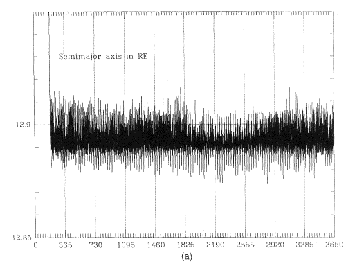
Figure 5a. The steady behavior of the semi-major eclipse of a 67-hour orbit over 10 years, after perturbations due to the Moon, Sun and the equatorial bulge of the Earth are taken into account. Its constancy tests the perturbation code.
|
This drift was eliminated by the algorithm of Bulirsch and Stoer, also given by Press et al. [1992]. That algorithm starts with a relatively crude variant of the Runge-Kutta integration, then subdivides the integration interval h and repeats the calculation, subdivides again with still smaller h and repeats again, until a number of such approximations is obtained, each with its step-size h. If one could use an arbitrarily small value of h, the result could be made arbitrarily accurate--but the calculation would be very long. Instead, one fits the results obtained with different values of h to a polynomial (a polynomial in h2 may be shown to suffice), and the results are then extrapolated to h=0. The limiting value obtained is surprisingly accurate.
Bulirsch-Stoer integrations of the orbit produced a steady unvarying value of the semi-major axis a (Figure 5a). In contrast, Mullins and Evans [1996] used Runge-Kutta integration and as shown in their figure (3a), in the course of 50 years their value of a slowly drifted. ENCKE2 repeated that calculation and found no drift, while completely matching their figures (3b) and (3c), suggesting that the drift in a did not invalidate their other results.
- As noted, three sources of perturbation were taken into account--Moon, Sun and the bulge of the Earth. The effects of the first two do not follow any simple pattern, but those of the bulge need to be handled with care.
Suppose the bulge were the only source of perturbation. Even with that perturbation, the gravity field is still axisymmetric, and therefore the orbit has a constant shape, in a plane which usually rotates slowly around the Earth's axis. Far from Earth, the perturbation is small and the field is well approximated by a gravitational monopole, so that one expects that part of the orbit to closely resemble a Keplerian ellipse. Near Earth, however, the orbit would significantly differ from an ellipse.
Thus, if one uses the local position and velocity at any instant to calculate an osculating ellipse (as was done here), the result will depend on the part of the orbit where the calculation was performed. Calculations far from Earth would yield very nearly the same osculating elements, e.g. the same semi-major axis a ; but calculations at points near perigee would give significantly different values. That systematic variation persists when perturbations due to the Moon and the Sun are added.
If orbital rectifications are performed whenever the appropriate criterion is satisfied, they will be randomly distributed around the orbit. Some will happen near perigee, and the osculating elements given by them would be quite inappropriate for most of the orbit, adding to the "random noise" in the output. A simple and effective remedy, practiced here, was to postpone any rectifications that were scheduled within a time T of a perigee pass, with T typically equaling 2 hours.
- In calculating the perturbations due to the Sun and the Moon, their positions need to be calculated for every point of the orbit. We used "low precision formulas" from the US nautical almanac, which give the Moon's position within 0.2 RE, while other celestial motions and times were derived using formulas by Meeus [1991]. These derivations can appreciably slow down the calculation--especially for the Moon, where even the simplified formulas involve 40 terms and 16 trigonometric functions. For both bodies, calculation time was greatly reduced by only deriving the positions of the Sun and the Moon every 12 hours, and interpolating in-between.
One caution must however be observed. Let A and B in Figure 5b be two positions of the Moon between which interpolation is performed, while O is the center of the Earth. If the interpolation is linear, since AB is a chord of the Moon's orbit, any interpolated point will always be closer to the Earth's center than the corresponding point on the actual orbit.
|
Figure 5b. The method used for interpolating positions of the Moon, between two calculated values A and B.
|
To avoid a systematic error from this cause, the actual interpolation was performed not between A and B but between A' and B', where the area of the triangle A'B'O equaled that of the orbital segment ABO, here approximated by a section of a circle. Stated in different terms, any linear interpolation between orbital points such as A and B is equivalent to approximating the orbital curve by a polygon. Here, instead of using an inscribed polygon, which will always be smaller than the actual orbit, we used a polygon of similar shape, but magnified by a factor f slightly larger than 1, giving it the same area as the actual orbit. All interpolated coordinates are then also multiplied by that factor f. That was the procedure adopted for the Moon: with the Sun, the angle AOB was so small that no such correction was necessary.
Launch Timing and Orbital Perturbations
The bottom curve in Figure 6 shows the predicted 10-year behavior of the radial perigee distance RP for a typical orbit, in this case with a period of 67 hours (apogee near 25 RE), launched due east from a site on the equator, longitude 40 W and with initial value RP = 1.1 RE. Figure 7 gives a magnified view of the first 1.5 years of that curve.
It is evident that perigee height undergoes three types of change: a semi-monthly wave of about 100 km peak-to-peak (PTP), a semi-annual one of about 850 km PTP, and a long scale irregular variation. All these changes reflect corresponding changes in the orbital eccentricity e. With a 20-RE apogee similar changes were observed, but their amplitude was reduced, so that the semi-annual wave was only about 600 km PTP.
Figure 6. Variation of the perigee height over a 10-year period, for orbits launched July 4, 2000, from initial perigee heights of 1.1, 1.3 and 1.5 Earth radii. Distances are in km. from the center of the Earth. Note the similarities in the semi-annual variation and the long-term trend.
|
Experimentation with orbits has shown that these curves are fairly robust: for instance, raising the initial perigee by 1000 km or by 2000 km yielded a very similar variation of the perigee height, but with all points lifted by about 1000 km (as in the higher curves of Figure 6). Thus given a satellite orbit starting with a given velocity from a predetermined perigee distance( e.g. from 7000 km, close to 1.1 RE), its subsequent perigee distances will depend on the phase of the launch date in the semi-annual perigee cycle.
If launch occurs at the peak of the cycle, perigee height on subsequent orbits will steeply decrease, and since the bottom of the curve is around 6150 km, the satellite will be lost. On the other hand, if launch is timed to be near the semi-annual minimum, the perigee height of later orbits will rise, and in the absence of other variations, it will not fall significantly below 7000 km.
Thus the first step in planning long-term missions is a fairly simple one. Using an orbital code, derive an orbit similar to the one being planned, starting slightly before the earliest acceptable launch date. Then plan the actual launch time around one of the minima of the semi-annual wave of perigee distance which you have obtained, giving two fairly broad launch windows per year, half a year apart. For even greater economy, one might launch around one of these minima at a time when the semi-monthly wave also hits minimum (see Figure 7). That can add nearly 100 km to the perigee altitude, but the launch window now shrinks to a day or two.
|
Figure 7. Magnified view of the first 18 months of the lowest trace in Figure 6. Note the semi-monthly variation..
|
In addition to the two periodic variations, a long-term trend also exists. In the example shown, perigee rises for two years, drops back over two years and then continues with milder changes. Some orbits display only minor changes, while others, like the one calculated by Mullins and Evans [1996], change quite dramatically. In particular, orbits near the critical inclination of i = 63.4° (arc sin 2/51/2) may evolve quite rapidly. For instance, the perigee of Russia's Interball-Tail satellite [Galeev et al., 1996], launched 3 August 1995 with i = 62.90, rose during the first year of the mission from its initial value of 7172 km to nearly 3 RE. Of course, such steeply inclined orbits slice through the plasma sheet almost perpendicularly, and spend relatively little time there.
Long-term trends also exhibit a certain amount of robustness, though one may have to experiment with several close orbits to see which fits best. The timing of the launch studied in Figures 6--July 4, 2000--is well-chosen, at the start of a rising trend. Launch in 2003, on the other hand, may encounter a trend of declining perigee, causing early loss, while the middle of 2005 is again at the bottom of a rising trend, albeit a milder one. The orbital inclinations to the equator and to the ecliptic, for the three orbits of Figure 6, are given in Figures 8a - 8b.
Eclipses and the angle χ
Eclipses are the bane of orbits with moderate inclinations to the ecliptic -- unfortunately, because these orbits also have the best plasma sheet coverage. Such coverage becomes even more important when one deals with a cluster or constellation of satellites, whose satellites should not only cover that region, but should do so concurrently.
Figure 8a. Ten-year variations of the inclination i to the Earth's equator in the three orbits in Figure 6.
|
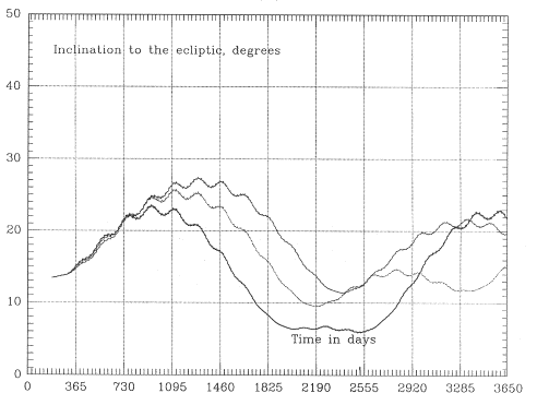
Figure 8b. Ten-year variations of the inclination ie to the ecliptic in the three orbits in Figure 6.
|
Figure 8c. Ten-year variations of the parameter χ in the three orbits in Figure 6.
|
The effect on distant eclipses due to variations of the conventional orbital elements (i, ω, Ω) is not easy to interpret intuitively, since a mixture of factors is involved. A much more intuitively significant parameter is the angle χ between the line of apsides--the long axis of the orbital ellipse--and the plane of the ecliptic; that is, (90-χ) is the angle between that line and the ecliptic pole. With χ less than 10° distant eclipses are likely, and when χ is close to zero they are at their maximum duration. Reducing the inclination ie to the ecliptic also tends to prolong distant eclipses, but χ is the main factor.
The strategies developed with Keplerian codes, seeking the fewest and shortest eclipses, practically assure that at the start of the mission χ is large. Unfortunately, after performing many orbital simulations, it was found that χ inevitably oscillates around χ=0, with a typical period between 5 and 15 years (Figure 8c gives the variation for the three orbits of Figure 6). Thus if we start at the peak of the cycle, χ will decrease and will typically pass χ=0 within about 2-3 years.
One could hope to improve the situation by "detuning" the orbit slightly, but that does not work out. The "reference orbit" has Ω=0. If one starts instead from Ω>0, the initial value of χ is already past its extremum and therefore reaches χ=0 even sooner than before. Starting with Ω<0 gives an initial value of χ preceding the extremum, so that more than a quarter-oscillation elapses before χ=0 is reached; however, the period of the oscillation is reduced, so that the total time elapsed from launch to the crossing of χ=0 stays about the same. Starting from latitude 10° instead of 5° will reduce the amplitude of those oscillations (reducing the average of χ and therefore increasing eclipse durations) but does not change their period.
In practice this seems to say that only the first year's passes through the tail will avoid long eclipses. A long term mission of this type is still feasible, but only if the spacecraft can survive intense chilling.
Fine-tuning the time of χ = 0
A method exists for moderating the effect of the passage through χ=0, but unfortunately the advantage gained is relatively slight.
Experimentation with orbits has shown that if the launch is delayed by half a year, the curve of χ against time t remains very similar, except that it is shifted ahead by half a year. Previously it was found that (for a given orbit) each year has two launch windows half a year apart, at the minima of the semi-annual variation in perigee height. They allow one to choose between two different times when χ=0, about half a year apart.
By launching from a site like Kourou at the "reference time" of the day, one assures that the satellite is in the tail around the summer solstice. By launching from a site south of the equator about 12 hours off the reference time, one obtains a "mirror image" orbit which passes the tail around the winter solstice, reaping similar benefits. Of course, changes in the right ascension of the ascending node shift that time, by the order of one month per year. Of the two launch windows, it is therefore preferable to choose the one which makes χ=0 occur when perigee is close to noon..
The time when χ=0 can be shifted somewhat by launching not due east, but at some small angle γ to the easterly direction, which increases the inclination i to the Earth's equator. For small values of γ, typically, every 5° in γ shifts the time of χ=0 by 2 months, which may be sufficient to assure that χ=0 occurs when apogee is at noon . Of course, orbits not launched in the easterly direction do not reap the full benefit of the Earth's rotation (408 m/s at Cape Canaveral, 465 m/s on the equator), but the penalty Δv is rather small:
|
γ | Δv |
|
|
|
5° | 1.548 m/s |
|
10° | 6.183 m/s |
|
15° | 13.868 m/s |
|
20° | 24.55 m/s |
The bad news is that the variation of χ near the time of χ=0 is not fast enough to avoid substantial eclipses. If χ=0 finds apogee at noon, it will be at midnight half a year before and after, at which time χ=2° and eclipses are still 6 hours long (whereas at χ=0 they would reach 9-10 hours).
Summary
A systematic procedure was developed to identify, evaluate and study orbits of scientific satellites that study the Earth's magnetosphere, in particular its plasma sheet and magnetotail. All these missions involve highly eccentric near-equatorial orbits, with initial perigee distances around 1.1 RE and typical apogee distances of 20-25 RE.
The selection and study of such orbits proceeds in three steps:
- Establish quantitative criteria or "metrics" by which the suitability of different missions may be compared. Such metrics also include all factors whose values determine the initial orbit
- Study the full range of available Keplerian orbits, to see which range of orbital elements best meets the criteria of #1.
- Simulate and study the evolution of the selected missions in subsequent years, due to gravitational perturbations by the Moon, Sun and the equatorial bulge of the Earth. Use such studies to improve strategies for selecting the mission.
In step #1, three types of metrics were particularly important:
(a) The mission should use inexpensive small spinning satellites, with their spin axis approximately perpendicular to the ecliptic. The orbits should require the smallest boost needed to achieve good coverage of the plasma sheet and of other interesting regions, give long lifetimes and avoid lengthy eclipses.
(b) The factors which affect the initial orbits are time of day of the launch, day of the year, and the year of launch itself. An option of launching into a parking orbit and then delaying the firing of the last stage was studied, as was the option of launching from sites other than Cape Canaveral and into directions other than due east.
(c) To evaluate coverage of various magnetospheric regions, subroutines were created which, given a point in space and some time, named the magnetospheric region in which the point was most likely located. Keplerian codes were then produced which tracked satellites hour by hour throughout the year, collecting statistics on region occupancy, eclipses and their durations, and other information.
Step #2
An important parameter in determining both coverage of the plasma sheet and eclipses was the orbital inclination ie to the ecliptic. A second factor was the time of the year in which apogee was at midnight, which because of the warping and hinging of the plasma sheet, greatly affected plasma sheet coverage. Using the Keplerian simulation described above, many such orbits were studied and their statistics were compiled and compared.
For launches from Cape Canaveral, the best orbits were obtained by sending the spacecraft into a parking orbit with moderately small ie and then waiting about a quarter of an orbit before firing the last stage, needed to achieve the final apogee. This method requires accurate 3-axis control in the parking orbit and was judged to be somewhat risky.
Orbits of much better quality--shorter eclipses, nearly twice the plasma sheet coverage and no need for a parking orbit--were obtained by shifting the launch site to latitudes 5°-10°. The orbits had ie of 13°-18° and apogee north of the ecliptic, covering midnight when the northward shift of the plasma sheet, due to the tilt of the Earth's magnetic axis, was at its maximum.
Step #3
In the long-term evolution of an orbit, it is important to avoid early atmospheric re-entry and long eclipses. One would furthermore like to preserve good plasma sheet coverage, but that in any case only changes slowly.
Early re-entry is avoided by launching at one of the semi-annual minima of the perigee distance, whose location can be establishing by examining a similar orbit starting a year or so earlier. A fairly long lifetime may be achieved by examining the long-term trend of perigee height (again, using a similar orbit for guidance) and timing the launch to coincide with a gradual rising trend in perigee height.
Avoiding distant eclipses is much more difficult. They depend most strongly on the angle χ between the ecliptic and the long axis of the orbital ellipse, and are worst near χ = 0. Unfortunately, on all orbits tested χ tends to oscillate with periods of 5-15 years, so that even if initially χ is close to its peak value, within 1/4 of a period χ=0 is crossed, producing long eclipses. One can ameliorate this problem by having χ=0 occur when apogee is near noon, but even then, half a year before and after that time χ is small enough to create problems.
Many of these problems are avoided by increasing ie, but then coverage of the tail is also greatly reduced, which is particularly unfortunate in a "constellation" mission of several spacecraft. The problem could also be solved by technology, if satellites could be designed that can endure the severe chilling of a 7-hour eclipse. For this one might even consider battery-free satellites which shut down completely in the Earth's shadow and "re-awaken" afterwards.
References
Battin, Richard H., Astronautical Guidance, xiv + 400 pp., McGraw Hill, New York, 1964.
Danby, John M.A., Fundamentals of Celestial Mechanics, 2nd edition, corrected and enlarged, xii + 483 pp., Willmann-Bell, Inc., Richmond, VA, 1992.
Fairfield, Donald H., Average and unusual locations of the Earth's magnetopause and bow shock, J. Geophys. Res., 76, 6700-6716, 1971
Galeev, A.A., Yu. I. Galperin and L.M. Zelenyi, The Interball Project to study Solar Terrestrial Physics, Kosmicheskiye Issledovania , 34, 339-62, 1996, English translation Cosmic Research, 34, 314-333, 1996.
Meeus, Jean, Astronomical Algorithms, iv + 429 pp, Willmann-Bell, Richmond, VA 1991.
Mullins, L.D. and S. W. Evans, The dynamics of the proposed orbit for the AXAF satellite, J. Astronaut. Sci., 44, 39-62, 1996
Press, William H., Saul A. Teukolsky, William T. Vetterling and Brian P. Flannery, Numerical Recipes,, 2nd ed., xxvi + 963 pp., Cambridge U. Press., 1992.
Sibeck, D.G., R.E. Lopez and E.C. Roelof, Solar wind control of the magnetopause shape, location and motion, J. Geophys. Res., 96, , 5489-95, 1991.
Smith, Bruce, Sea Launch Mission to Demonstrate System, Aviation Week & Space Technology, p. 74-78, March 22, 1999a
Smith, Bruce, Sea Launch Passes Demonstration, Aviation Week & Space Technology, p. 65, April 5, 1999b
Stern, David P., Planning the "Profile" Multiprobe Mission, p. 136-141 in Science Closure and Enabling Technologies for Constellation Class Missions, V. Angelopoulos and P. V. Panetta, eds., Berkeley Univ., 1998a. [Also: http://www.phy6.org/profile/Monogr1.htm]
Stern, David P., Science tasks for "Profile", p. p. 66-71 in Science Closure and Enabling Technologies for Constellation class Missions, V. Angelopoulos and P. V. Panetta, eds., Berkeley Univ., 1998b. [Also: http://www.phy6.org/profile/Monogr2.htm]
Stern, David P. and Mauricio Peredo, "The Exploration of the Earth's Magnetosphere," textbook on the world-wide web, http://www.phy6.org/ /Education/Intro.html .
Stern, David P. and N.F. Ness, Planetary magnetospheres", Ann.Rev. Astron. Astrophys., vol. 20, 125-138, 1982.
Tsyganenko, N.A., Modeling the Earth's magnetospheric magnetic field confined within a realistic magnetopause, J. Geophys. Res., 100, 5599-5612, 1995.
Back to the "Profile" Index Page
Back to the "Exploration" Index Page
|
Author and Curator: Dr. David P. Stern
Mail to Dr.Stern: audavstern("at" symbol)erols.com
Placed on the internet 21 January 2006
|